ROBOTICS · WEIGHT EDITING · AUTORESEARCH

We Asked Opus-5.5 to Edit π0.5’s Weights. AutoResearch Made It Happen.

Two findings: a RoPE-based route to faster robot actions and an unexpected RTC prefix bug.

Ziyang Gong1,2 · Kaifeng Zheng1,2 · Yingrui Huang1 · Wendi Chen1,2 · Jiaguo Tian1,2 · Junkai Yang1,2 · Minghuan Liu1 · Zhenjie Yang3
1 Shanghai Innovation Institute2 Shanghai Jiao Tong University3 The University of Hong Kong

One Frontier Model. One policy.
Two weight edits.

One Frontier ModelOpus 5.5
One robot policyπ₀.₅
One GPURTX 4090
~111 minutesOffline research
−12.0%Mean bottle time at 40 Hz · 17.99 → 15.83 s
−89.8%Mean chunk jump across 30/35/40 Hz · 30.88 → 3.14 mm

Recent progress in Weight Editing made us wonder: when a Frontier Model directly edits the weights of a trained robot policy, how does it find changes that work? We gave Opus-5.5 the task of making a robot move faster by editing its policy’s weights. What followed was an AutoResearch process of forming hypotheses, running experiments, and revising its approach after failures.

Opus proposed that RoPE action positions could influence motion timing, tested that hypothesis, and fitted the useful intervention into Q/K weights. It also found an unexpected prefix-handling bug and encoded a repair in the time-modulation weights. In our real-robot bottle-placement tests, both the original and edited policies achieved a 100% success rate, while the edited policy achieved consistently shorter completion times at action execution frequencies of 30, 35, and 40 Hz: 4.3%, 7.4%, and 12.0% reductions against the original policy at each matched rate. Across the three rates, mean chunk jump fell from 30.88 to 3.14 mm, a reduction of 89.8%. The improvement in chunk jumps does diminish as execution frequency rises: 94.5% at 30 Hz, 90.7% at 35 Hz, and 85.2% at 40 Hz.

Opus demonstrated a strong understanding of parameter space. But we believe the success of these edits depended not only on parameter editing itself, but to a greater extent on its AutoResearch ability to discover problems, design experiments, and solve them.

THEN WE TESTED IT ON YAM

Original vs. edited at 30, 35, and 40 Hz.

30 Hz−4.3%Mean time

22.42 → 21.46 s

35 Hz−7.4%Mean time

19.43 → 17.99 s

40 Hz−12.0%Mean time

17.99 → 15.83 s

30 Hz → 40 Hz−29.4%Mean time · original → edited

22.42 → 15.83 s

Weight editing + higher execution rate
Both achieved 100% success in these trials

Same layout, three runs per condition. The values above compare mean completion times, original → edited. The video first compares all three original 30 Hz runs with all three edited 40 Hz runs, then shows the median-duration original run and the fastest edited run at each of 30, 35, and 40 Hz.

Top: original TT-RTCBottom: combined edit
1× playback. 0:00: original 30 Hz vs. edited 40 Hz (columns: repeats 1–3). From 0:23: same-rate comparisons (columns: 30, 35, and 40 Hz). Each segment starts at formal rollout start; each view freezes at the fourth bottle release. Timers show elapsed time within each run.

Beyond bottles: coin grasp-to-handover time decreased by 20.7%; block stacking showed no clear speedup. These are initial, task-dependent gains.

FINDINGS / What Opus found

Two weight edits: a speedup and an unexpected bug fix.

A prefix bug left unhandled in the official Training-Time RTC implementation, and a RoPE intervention for action timing. Opus addressed both through new weights, keeping the production inference code unchanged.

1 × RTX 4090Offline research onlyNo robot interaction
01 / PREFIX REPAIRUNEXPECTED FINDING

A prefix bug left unhandled
in the official Training-Time RTC.

Each denoising iteration first restores the conditioned prefix. But the final iteration updates it once more using the predicted velocity, then returns without restoring it again. Here velocity means the flow-matching update, not physical robot speed. If inference returns before the reserved prefix runs out, modified prefix actions can enter execution. The official fixed-delay example discards the whole prefix, so this issue is not exposed.

How Opus edited the time-modulation weight

  1. Choose the zero-update target

    Set scale to −1 so the action features cancel out. Choose shift = s* so the unchanged output layer produces zero.

    s∗Wout+bout=0
  2. Apply the change only at t = 0

    Let d be target minus original modulation. Solve for u using time features cₜ: enable d for the prefix and suppress it at the ten sampling times.

    c0u=1,ctu=0
  3. Write the increment into W

    Take the outer product to obtain ΔW. Since cₜΔW = (cₜu)dᵀ, the fixed weight edit carries the time-dependent switch.

    ΔW=udT,W′=W+ΔW

The equivalent code change: one prefix-restoration line

Before · source excerpt (omissions marked)
guided, model_input, time = sampling_input(x, target, omega, sigma, config)
return guided - predict_velocity(model_input, time) / num_steps
# ...
return jax.lax.fori_loop(0, num_steps, step, noise)
Equivalent code fix · one restoration line
actions = jax.lax.fori_loop(0, num_steps, step, noise)
actions = omega * target + (1 - omega) * actions
return actions

The core code repair is one line: restore the conditioned prefix after the sampling loop. With a hard 0/1 mask, the highlighted line is equivalent to actions[:, :6] = target[:, :6]. The other lines collect and return the result. This is an equivalent code control; Opus delivered edited weights that make the prefix update nearly zero, without adding this operation to production inference.

Actual weight-edit code · closed-form solve
Original script: K = article W; W = article W_out
u = np.linalg.lstsq(A, rhs, rcond=1e-10)[0]
s_star = -np.linalg.lstsq(W.T, bo, rcond=None)[0]
d = np.concatenate([-1. - scale0, s_star - shift0, np.zeros(1024)])
dK = np.outer(u, d)
K2 = K + dK

A stacks time features, rhs selects the prefix, and scale0/shift0 are the original modulation. K changes; W and the inference code stay fixed.

Median offline transition distance

Original19.16 mmWeight repair1.80 mmCode fix1.88 mm

Finding: on the same offline inputs, the weight repair and the one-line code repair reduced transition distance to similar levels. Opus identified the prefix inconsistency and approximately encoded its repair in the final normalization layer’s time-modulation weights.

02 / RoPE TEMPO ACCELERATIONACTION TIMING → WEIGHTS

Increase RoPE position spacing.
Encode the effect in the weights.

Opus tested a change from P + i to P + si while keeping execution at 30 Hz. At s = 1.25, the median offline path progress ratio was 1.131, with 1.229 mm deviation.

action_positions = P + 1.25 * i

Measured offline diagnostics: more spacing is not always better

Path progress ratio ↑
0Dashed line: original = 1s=0.8: 0.851 ×0.8510.8s=1.25: 1.131 ×1.1311.25s=1.5: 1.175 ×1.1751.5s=2.0: 1.009 ×1.0092.0RoPE position scale s
Path deviation (mm) ↓
0s=0.8: 0.793 mm0.7930.8s=1.25: 1.229 mm1.2291.25s=1.5: 1.935 mm1.9351.5s=2.0: 4.674 mm4.6742.0RoPE position scale s

Direct RoPE intervention · 58 valid observations out of 60 · median across observations. The green bar marks the selected s = 1.25. These are predicted-path metrics, not real-robot completion speed.

Fit the RoPE effect into Q/K weights.

The position intervention becomes a teacher. Opus constructs rotated Q/K targets and solves for new projection weights in layers 1–17, so the candidate can retain the original inference code and position rule.

Position intervention → equivalent rotation → fitted weights

The following is simplified pseudocode. Rotating pre-RoPE Q/K by the extra angle is algebraically equivalent to the teacher position change; a shared fitted projection only approximates that rotation.

Original
q = X @ Wq
k = X @ Wk
Q = rope(q, P + i)
K = rope(k, P + i)
Teacher · position-rule change
q = X @ Wq
k = X @ Wk
Q = rope(q, P + 1.25 * i)
K = rope(k, P + 1.25 * i)
Candidate · only new weights
q = X @ Wq_fit   # new weights
k = X @ Wk_fit   # new weights
Q = rope(q, P + i)  # original positions
K = rope(k, P + i)

How Opus constructed Y and fitted ΔW

  1. Collect hidden features X

    Run local demonstrations and historical rollout observations through the model. Stack the hidden features entering each Q/K projection into X.

    Q/K0=XW0
  2. Rotate the original Q/K to obtain Y

    For action i, apply an extra RoPE rotation for position offset 0.25i to the original projection of the same feature. This supplies the gap from P+i to P+1.25i. Stack the target vectors as rows of Y.

    yi=R(0.25i)(W0Txi)
  3. Fit W, then subtract the original

    Fit XW to Y, regularizing toward W₀. Apply this separately to Q and K in layers 1–17; inference keeps the original RoPE.

    Wfit=arg⁡minW[∥XW−Y∥F2+λ∥W−W0∥F2]
ΔW=Wfit−W0,W′=W0+ΔW

Offline path progress (original = 1)

Original1.000×Tempo acceleration only1.199×Deviation1.08 mm
On this page

The Full Blog

Abstract

Robot policies trained by imitation often inherit the execution tempo of their demonstrations. Yet task semantics, skills, and key interactions can exhibit a degree of temporal invariance. For example, watching the same skill tutorial at 3× or 0.5× speed changes its pace while preserving the core skill knowledge it conveys. Motivated by this idea, we explored whether a Frontier Model could adapt the weights of a trained robot policy to control its execution tempo while retaining task knowledge and manipulation capabilities. Our aim was faster, smoother closed-loop execution while respecting robot dynamics and preserving task success. We gave Opus 5.5 a pretrained π0.5 policy, source code, historical trajectories, and one RTX 4090, requiring a reversible checkpoint without backpropagation or production-code changes. It hypothesized that RoPE action-position spacing influences predicted motion, tested this through controlled experiments, and fitted Q/K projections to approximate the intervention after output-layer fitting failed to generalize. It also discovered an unexpected prefix-handling issue and derived a separate weight edit to reduce chunk jumps. In our real-robot tests at 30, 35, and 40 Hz, mean bottle-placement time decreased by 4.3%, 7.4%, and 12.0% relative to the original policy at each matched rate; mean chunk jump decreased by 89.8% when averaged equally across the three rates. Attention-region interventions showed that action-to-action score changes retained much of the offline progress gain. Beyond these initial performance gains, we examine the research process: mechanistic understanding, hypothesis formation, experiments, and revision after failure. This case offers a concrete view of how Frontier Models might participate in discovering and solving problems in embodied intelligence.

1 Our Idea and Research Setup#

We asked whether a Frontier Model could understand the parameters of a trained robot policy and, through a small number of edits, make the robot execute actions and complete tasks faster. We gave this problem to Opus 5.5, asking it to derive weight changes from mechanisms and objectives.

We provided the objective and environment; Opus 5.5 proposed hypotheses, designed experiments, and selected a solution. It worked through Claude Code with one NVIDIA GeForce RTX 4090, a trained π0.5 [2] Training-Time RTC checkpoint, model and inference code, and recorded YAM demonstrations and rollouts. Opus never operated the robot or received online physical feedback; its research used only existing recordings. We conducted the subsequent physical tests on YAM arms. It surveyed 136 historical rollouts (5 task types) and 154 human demonstrations (3 task types). For editing, it selected a separate set of 12 demonstrations (6 task types) and 12 rollouts (4 task types) from the available data, covering coin insertion, moving-block picking, stacking, bottle placement, and clock manipulation.

We prohibited backpropagation, gradient-based optimizers, and LoRA, while allowing forward-pass experiments and closed-form fitting. We asked it to change as few parameters as possible, preserve the production inference and control programs, and deliver an independent checkpoint that could be rolled back. A 20%–30% reduction in task time was the exploratory target; a stable 5%–10% improvement would also be meaningful. It needed to check smoothness and cross-task behavior, and compare against the original policy, action-amplitude scaling, trajectory time scaling, and random weight edits.

The resulting method developed through mechanistic hypotheses, controlled experiments, and revisions. We are interested not only in performance after editing, but also in how Opus identified problems, tested explanations, and changed direction after failure. Section 2 presents its research process; Section 3 reports our additional real-robot and mechanistic experiments. We close by considering what this case suggests about AutoResearch in robotics.

Here, an action chunk is a policy prediction of 50 future action steps. Each action step contains 12 joint targets for the two arms and 2 gripper targets. The baseline action execution rate is 30 Hz; Section 3.1 also tests 35 and 40 Hz. We execute 32 steps per cycle. When updating the plan, the first 6 steps of the old plan serve as conditioning actions, or the RTC prefix. We call an abrupt change in target position at a plan switch a chunk jump; this describes a change in commands, not an instantaneous movement of the physical arm.

2 Opus 5.5’s Hypotheses, Experiments, and Solution#

2.1 Locating the Opportunity: Inference Waiting or Action Execution?#

Opus 5.5 first checked whether task duration was dominated by waiting for model inference. It read the deployment configuration and compared inference times, action commands, and measured joint states across 136 historical RTC trajectories. Each inference took approximately 105–109 ms, substantially less than the roughly 1.073 s plan-update period. The recordings also showed no obvious idle intervals dominated by waiting for the next inference. It then used action speeds and pauses in 154 demonstrations as a reference and turned to the actions generated by the policy.

This diagnosis focused the investigation on saving time during action execution. Opus 5.5 pursued two lines of inquiry: first, whether anomalies at old-to-new chunk transitions originated in generation; second, whether subsequent actions could advance farther while preserving the task path. The first led to prefix repair, and the second to tempo acceleration through a Q/K projection edit; we refer to their combination as the combined edit.

2.2 Repairing Chunk Jumps in the Retained Action Prefix#

By comparing model outputs with executed commands, Opus 5.5 found that the first 6 steps were supplied as conditioning actions, but the generated outputs deviated from those old actions. Deployment usually discarded only the first 4 expired steps, so deviations in steps 5 and 6 entered execution. The cause was that the prefix was not restored again after the final flow-matching integration step.

Opus 5.5 computed a weight-update matrix ΔW and saved W′=W+ΔW in a new checkpoint. Opus edited W, the linear-layer weight mapping time features to scale and shift in the final normalization layer (Figure 1; final_norm_1.Dense_0.kernel). The 1024×3072 matrix ΔW specifies an increment for every weight. The goal is nearly zero prefix updates while preserving outputs at other sampling times, with inference code unchanged.

Prefix repair changes only the green time-projection layer to \(W'\) . Time features \(c_t\) modulate action features \(x_t\) at final normalization; the action-output projection stays fixed.
Figure 1. Prefix repair changes only the green time-projection layer to W′. Time features ct modulate action features xt at final normalization; the action-output projection stays fixed.

The original time-modulation process is shown in Figure 1, using W at the highlighted location. The prefix uses generation-time condition t=0; other actions use 1.0,0.9,…,0.1. This is not physical execution time. Time encoding and time_mlp_in/out map t to 1024-dimensional features ct; c0 is not zero. For one action token, let xt be its hidden features after 18 Transformer blocks, and mt the three groups of modulation values from the time branch. Features in this subsection are row vectors; u,d are column vectors. The original model adjusts xt using scale and shift: mt=[scalet,shiftt,gatet]=ctW+b,xout,t=RMSNorm(xt)⊙(1+scalet)+shiftt,vt=xout,tWout+bout.(1) These are existing model operations, which Opus used to derive the edit. Here, ⊙ means elementwise multiplication; gate is unused. RMSNorm(x)=x/mean(x2)+10−6 contains no additional learned scale; time modulation is written separately. The linear layer action_out_proj, with Wout,bout, has Wout∈R1024×32 and produces the sampling update vt∈R32; it is not the time MLP. The prefix repair replaces only W, preserving b,Wout,bout.

Step 1: choose targets that give zero prefix updates. Primes denote edited quantities. Opus targeted scale −1 and solved for the minimum-norm s∗ that gives zero after the linear action output layer: scale0′=−1,shift0′=s∗,s∗Wout+bout=0,xout,0′=RMSNorm(x0)⊙0+s∗=s∗,v0′=0.(2) The Transformer output x0 need not be zero: the target scale removes its influence, while the target shift makes the final features equal to s∗ and cancels the output bias.

Step 2: compute the target modulation change. Subtracting original values from targets gives dT; adding it back verifies the desired result: dT=[−1−scale0, s∗−shift0, 0],m0+dT=[scale0,shift0,gate0]+dT=[−1,s∗,gate0].(3) Step 3: solve for u to apply the increment only to the prefix. Opus stacked the time features at the ten sampling times and at the prefix condition t=0 as rows of A∈R11×1024. It sought 1024 coefficients u giving c0u=1 for the prefix and ctu=0 at the ten other times. Stacking these targets into r yields A=stackrows(c0,c1.0,c0.9,…,c0.1),r=(1,0,…,0)T,u=argminz∥Az−r∥22(minimum-norm solution).(4) A dot product of 1 adds the full change dT to the prefix; a dot product of 0 adds nothing. Thus c0 comes from the original model, whereas u comes from this solve.

Write the weights and check the effect. The desired change after applying the new weights is (ctu)dT. By associativity, this equals ct(udT), so udT can be added directly to the weight matrix: ΔW=udT,W′=W+ΔW,Wij′=Wij+uidj,ctΔW=ct(udT)=(ctu)dT,mt′=ct(W+ΔW)+b=mt+(ctu)dT.(5) Row i of ΔW is uidT: all rows are scaled copies of the same vector, leaving only one independent direction. This is a rank-one update.

Across 36 demonstration observations and 24 historical execution observations, the prefix joint error fell from approximately 0.095 rad to 4.49×10⁻⁴ rad. The maximum change in subsequent actions was approximately 0.0034 rad, with almost no change in path progress. Opus 5.5 therefore retained this prefix repair and continued searching for a speedup method. Our code audit and experiments on this issue appear in Section 3.2.

2.3 The Action-Tempo Hypothesis and RoPE Position Intervention#

The prefix repair did not make subsequent actions advance faster. While reading the model code, Opus 5.5 proposed a hypothesis for acceleration: “My leading hypothesis is that action timing depends on RoPE positions.” We elaborate on this hypothesis as follows: the model may have learned an implicit relationship between action-position spacing and action displacement; increasing the internal position spacing while keeping the physical control interval unchanged may increase useful displacement over the same duration.

Figure 2 summarizes the intervention: change the coordinates used to read the action sequence, then test whether predicted actions advance faster.
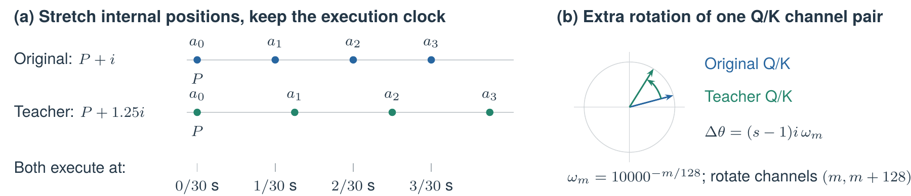
RoPE intervention: internal action-position spacing increases while the execution clock stays fixed. Each Q/K channel pair receives an extra rotation; the circle is schematic.
Figure 2. RoPE intervention: internal action-position spacing increases while the execution clock stays fixed. Each Q/K channel pair receives an extra rotation; the circle is schematic.

Implementation: change the Q/K rotations associated with action positions.

Let i=0,…,49 index actions and P denote the number of unmasked context tokens. Action indices here and in the subsequent offline formulas are zero-based. The internal positions change, while the physical execution interval remains Δt=1/30 s: pi=P+i,pi(s)=P+si,tiexec=t0+iΔt.(6) RoPE encodes position through rotations of Q/K [3]: qi=WQTxi,ki=WKTxi,Qi=R(pi)qi,Ki=R(pi)ki.(7) Here, xi∈R1024 is the column-vector feature after the layer’s adaptive normalization and before Q/K projection. WQ,WK∈R1024×256 denote the weights for one query head and the shared key head; the implementation has eight query heads and one key/value head. Within each 256-dimensional head, channels m and m+128 form a rotation pair, for m=0,…,127. For one such pair (a,b), [a′b′]=[cos⁡θ−sin⁡θsin⁡θcos⁡θ][ab],θ=p10000−m/128.(8) R(p) denotes the rotations of all 128 channel pairs. Holding the content vectors before rotation fixed, the inner product between actions i,j changes from the original expression to QiTKj=qiTR(j−i)kj,(Qi(s))TKj(s)=qiTR(s(j−i))kj.(9) The intervention therefore increases relative position spacing between actions. It also changes how action queries read the unchanged image, text, and state keys. Through softmax and the weighted aggregation of V, these changes affect subsequent action generation. The intervention does not directly scale V or joint targets.

Test: does the position intervention increase progress along the original route?

Opus 5.5 ran two sets of controls: (1) on 36 demonstration observations and 24 historical rollout observations, it changed action positions in all 18 layers to P+si, testing s=0.8,1.25,1.5,2.0; (2) on 36 demonstration observations, it kept RoPE unchanged and accelerated only the first six conditioning actions by factors of 1.25, 1.5, and 2.0. Each intervention and the original model used the same observations and initial noise.

It first resampled the original predictions at different speeds and found the speed that most closely matched the intervened joint trajectory. The RoPE intervention with s=1.25 corresponded to approximately 1.12×, whereas accelerating only the prefix corresponded to approximately 1.01×. It therefore continued to investigate the position intervention.

Opus 5.5 then tested: at the same action step, does the edited model move farther along the route planned by the original model? At a fixed action execution rate, the same step corresponds to the same elapsed execution time. It performed forward kinematics and connected the positions of the original TCP poses into a reference route. Each edited position was matched to the nearest point on that route. Dividing the cumulative distance along the route to that point by the original model’s distance at the same action step gives the path-progress ratio; the mean nearest distance from edited positions to the route gives the path deviation (Figure 3).
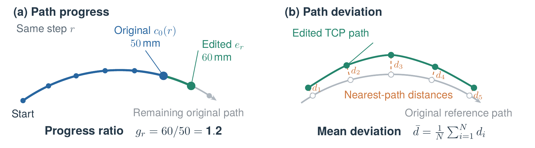
Two path metrics. (a) At the same time, the original model has advanced 50 mm, while the edited position corresponds to 60 mm along the reference route, giving a progress ratio of 1.2. (b) Averaging the nearest distances from edited positions to the reference route gives the path deviation.
Figure 3. Two path metrics. (a) At the same time, the original model has advanced 50 mm, while the edited position corresponds to 60 mm along the reference route, giving a progress ratio of 1.2. (b) Averaging the nearest distances from edited positions to the reference route gives the path deviation.

The calculation excludes the first six conditioning steps. Let cref(u) be the linearly interpolated reference TCP route from original steps 6–49 (in meters), Lref(u) its cumulative arc length from step 6, and er the edited position at step r. Progress is evaluated only at r=21,37; deviation uses all positions in I={6,…,37}. Matching the code, progress searches the grid Up={6+0.01k:k=0,…,4300}; deviation searches Ud, comprising 880 equally spaced points over [6,49]: ur∗=arg⁡minu∈Up∥er−cref(u)∥2,r∈{21,37},gr=Lref(ur∗)max{Lref(r),10−9},d¯=1000|I|∑r∈Iminu∈Ud∥er−cref(u)∥2.(10) The denominator floor is 10−9 meters, avoiding division by zero when reference progress vanishes; the factor of 1000 converts d¯ to millimeters. Table 1 reports g37 and d¯ (mm). Arms whose original motion covers less than 15 mm within the comparison interval are excluded. Eligible arms are averaged within each observation, followed by the median across observations.

Table 1. Position scaling versus prefix acceleration. Opus 5.5 saved per-sample metrics; we report medians over eligible observations: 58 of 60 inputs in the RoPE group and 34 of 36 in the prefix group.

Intervention Scale Eligible observations Progress ratio Path deviation
Action RoPE 0.80 58 0.851 0.793
Action RoPE 1.25 58 1.131 1.229
Action RoPE 1.50 58 1.175 1.935
Action RoPE 2.00 58 1.009 4.674
RTC prefix time compression 1.25 34 1.004 0.492
RTC prefix time compression 1.50 34 1.004 0.796
RTC prefix time compression 2.00 34 1.007 1.134

Table 1 shows that s=1.25 and 1.5 increase progress, whereas the benefit largely disappears at 2.0 and deviation increases. Accelerating only the prefix has little effect. We hypothesize that the relationship between action positions and displacements learned at a fixed action execution interval may limit the benefits of increasing position spacing. This is an interpretation of the non-monotonic trend, rather than an established cause.

Opus 5.5 selected s=1.25 as its main target. This intervention changes the position rule within the action expert’s attention, leaving its weights unchanged. To preserve the production inference code, it used this model as a direct RoPE teacher and attempted to internalize the intervention into new weights with the same architecture as the original model.

2.4 First Attempt: Fit Only the Final Action Output Layer#

The minimal-change test: can editing only the last layer reproduce the teacher’s final actions? The original output weight is 1024×32: the first 14 channels represent the two arms and grippers, and the remaining 18 are padding. Opus 5.5 fitted only the first 14 columns, preserving the other columns and all biases. Below, B∈R1024×14 denotes those columns and b0∈R14 the corresponding bias; AiT,zk,i,vk,i∈R14 contain those 14 channels in normalized action space. AiT is the teacher’s final output, zk,i the candidate state at iteration k and position i, and hk,i∈R1024 the column-vector feature after final time-conditioned normalization, entering the output layer. The remaining generation time is σk=1−k/10: vk,i∗=zk,i−AiTσk,vk,i=BThk,i+b0,zk+1,i=zk,i−0.1vk,i,k=0,…,9,i≥6.(11) v∗ is the target update toward the teacher’s final action, not the robot arm’s velocity. Opus 5.5 fitted B using least squares regularized toward the original weights, with bias b0 fixed. The sampler iterates ten times to produce the final actions (Figure 4).
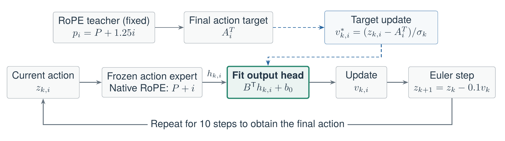
Fit only the green output layer using targets derived from the teacher’s final actions. Its predictions drive the 10-step sampler; all other weights and native RoPE remain fixed.
Figure 4. Fit only the green output layer using targets derived from the teacher’s final actions. Its predictions drive the 10-step sampler; all other weights and native RoPE remain fixed.

Reconstruction on fitting inputs and transfer to new inputs were checked separately. Let ai,j,ai,jT be the candidate’s and teacher’s final joint targets, with j ranging over the 12 joints. The joint error for each observation is ERMS=132×12∑i=637∑j=112(ai,j−ai,jT)2.(12) This squares the errors, averages them, and takes the square root, giving an error in radians; results are then averaged over observations. To check for abrupt changes in motion, it computed jerk, the rate of change of acceleration, from TCP positions pi: ji=pi+3−3pi+2+3pi+1−piΔt3,J=129∑i=634∥ji∥22.(13) The reported ratio is Jedit/Jorig, averaged over eligible arms within each observation. It excludes chunk transitions and is interpreted together with path progress and deviation.

After three fitting rounds on 24 demonstration observations, joint RMS was 0.0050 rad. On another 12 demonstration and 16 historical rollout observations, the error increased to 0.0239 rad, mean path deviation was 8.256 mm, and the jerk ratio was 3.245. Reconstruction quality did not carry over to the test inputs, so Opus 5.5 abandoned output-head fitting and turned to the attention layers.

2.5 Moving Inside Attention: Fitting Q/K Projections#

Opus 5.5 moved the fitting target from final actions to Q/K representations: a known rotation directly supplies the targets, which the new weights approximate (Figure 5).
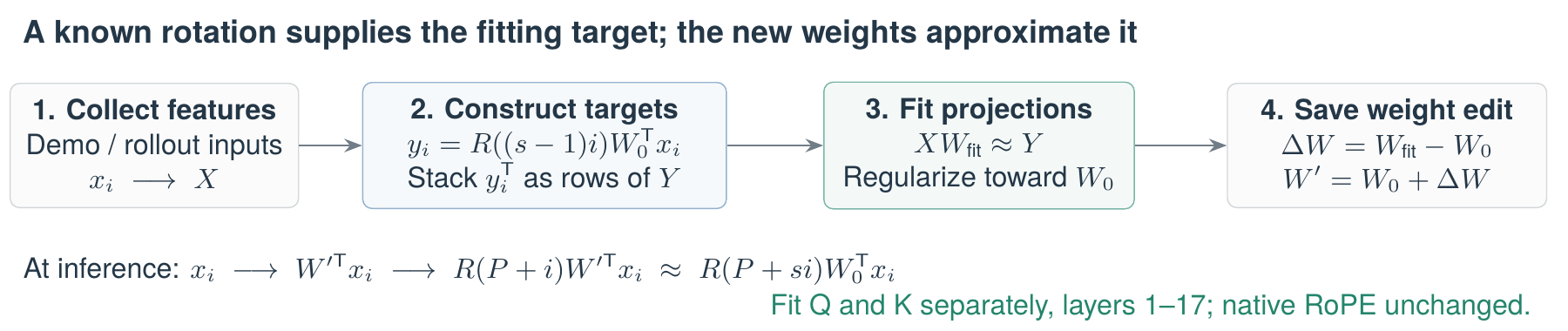
Construct \(Y\) by rotating the original Q/K projections of the same features, then fit and save new weights. Native RoPE remains unchanged at inference.
Figure 5. Construct Y by rotating the original Q/K projections of the same features, then fit and save new weights. Native RoPE remains unchanged at inference.

Step 1: construct intermediate representation targets. To retain the candidate’s native RoPE R(P+i) while approximating the teacher’s R(P+si), an additional rotation must be supplied by the projection output: R(P+i)R(δi)=R(P+si),δi=(s−1)i.(14) Targets are therefore constructed separately for Q and K: yiQ=R(δi)WQ,0Txi,yiK=R(δi)WK,0Txi.(15) Each target yi comes from applying a known rotation to the original Q/K of the same hidden feature xi, without human labels for faster actions.

Step 2: collect features and fit a closed-form solution. Opus 5.5 first checked whether the feature-collection forward pass altered the original output. Joint RMS was approximately 0.00037–0.00044 rad, below its chosen tolerance of 0.002 rad. It transposed the column vectors, using xiT and yiT as individual rows of X∈RN×1024 and Y∈RN×256, then solved Wfit=arg⁡minW(∥XW−Y∥F2+λabs∥W−W0∥F2)=(XTX+λabsI)−1(XTY+λabsW0),ΔW=Wfit−W0,λabs=λgridtr(XTX)1024.(16) The first term brings the new projection closer to the target; the second limits its departure from the original weights. Here, ∥⋅∥F2 is the sum of squared entries, I is the identity matrix, N is the number of collected feature rows, and λgrid is the candidate regularization coefficient, scaled by feature energy. The implementation solves a linear system rather than explicitly computing an inverse and uses no backpropagation. Each round recollects features from the candidate and accumulates XTX and XTY across rounds before solving; X,Y denote the accumulated samples. V projection weights remain unchanged. The shared weights do not directly receive the action index, so they rely on position information already present in the features to approximate the additional rotation.

Step 3: inspect generated actions and refine the fit. The initial fit edited Q/K in all 18 layers. After two rounds, normalized action RMS against the teacher on fitting observations fell from 0.03694 to approximately 0.00298. This measured final actions, not Q/K feature errors. The refined fit preserves layer 0 and fits only layers 1–17; its corresponding teacher also changes RoPE only in those layers. The rationale was that layer 0’s inputs have not yet undergone action-attention mixing and may lack the information needed for a shared projection to distinguish action indices.

Step 4: validate the refinement on held-out observations. The tempo edit used 48 observations from 12 demonstrations and 12 historical rollouts for fitting, reserving another 36 time points for testing. The time points do not overlap, but come from the same trajectories. After three fitting rounds, on the shared test set, the progress ratio increased from approximately 1.17 for the initial version to 1.20, deviation fell from 1.26 to 1.08 mm, and the jerk ratio fell from 1.47 to 1.37. Opus 5.5 therefore retained the tempo edit and proceeded to test edit strength and its combination with prefix repair.

2.6 Adding Parameter Constraints and Testing the Combination with Prefix Repair#

Opus 5.5 controlled the fitted change with an editing strength α: W(α)=W0+αΔW,ΔW=Wfit(s=1.25)−W0.(17) α=0 gives the original Q/K projections, and α=1 gives the full tempo edit. This is a different parameter from the positional scale s=1.25 used during fitting. When it tested α from 0.25 to 1.5, progress initially increased, then saturated as path deviation grew. Restricting the edit to rank 16, 64, or 256 gave progress ratios of approximately 1.06, 1.10, and 1.16, below the approximately 1.20 achieved by the full tempo edit.

It then compared prefix repair, tempo edit, and their combination on the same 36 test observations, adding trajectory time scaling and action-amplitude scaling as baselines, both with a factor of 1.21445. The path and jerk metrics in Table 2 include 35 valid observations. The chunk-jump metric is the maximum adjacent TCP displacement around the splice between the first 4 steps of the old plan and steps 5–13 of the new plan, taking the larger value across the two arms. It includes ordinary displacement between adjacent actions.

Table 2. Offline comparison on identical test inputs. All metrics are medians; progress, deviation, and jerk use 35 valid inputs, and chunk jump uses 36. A progress ratio of 1.214 means advancing farther along the original path in the same time, not a 21.4% reduction in successful task completion time.

Method Progress ratio Deviation (mm) Jerk ratio Chunk jump (mm)
Original 1.000 — 1.000 44.223
Prefix repair only 1.000 0.178 1.004 5.822
tempo edit only (α=1) 1.199 1.076 1.367 41.453
Combined edit 1.214 1.071 1.363 5.442
Trajectory time scaling 1.257 0.038 0.827 44.223
Action-amplitude scaling 1.054 4.870 1.217 53.529

The combined candidate increased path progress and reduced chunk jumps, but its within-chunk jerk ratio rose to 1.363. Time scaling had lower deviation and jerk, but retained the original chunk jumps. A random weight direction produced 24.05 mm path deviation and a jerk ratio of 31.07, failing to preserve the original behavior. Opus 5.5 ultimately selected the combined edit with α=1. Since it did not compare against prefix repair combined with time scaling, this does not establish that editing outperforms every post-processing alternative.

2.7 Deliverables and Research Cost#

After checking saving, rollback, and native reloading, Opus 5.5 delivered an independent checkpoint that modified 1.16% of all model parameters. All 8 test inputs produced valid outputs. Its initial research run took 1 hour, 50 minutes, and 42 seconds, with 193 tool calls (163 Bash, 18 Write, 8 Read, and 4 others) and 187 API requests. Usage records were available for 181 requests, totaling 184,614 output tokens, with 433,426 cache-write tokens and 36,783,281 cache-read tokens. The 6 requests without usage records are not counted as zero; cache reads include repeated context. These figures exclude subsequent real-robot analysis and preparation of this article.

3 Our Follow-up Experiments and Analysis#

We next measured actual task time and chunk jumps, and analyzed internal effects through attention-region interventions and prefix-handling controls. These are our additional experiments and are not included in the cost of Opus 5.5’s initial research run.

3.1 Real-Robot Experiments: Task Time and Action Quality#

We compared the original Training-Time RTC policy with the combined edited policy (α=1) on bottle placement, coin insertion, and block stacking. Within each task, the two policies were evaluated on the same object layout, with three executions per condition. Only bottle placement was tested at multiple action execution rates. (1) Bottle placement: weight-editing gains persist across execution rates. Beyond the earlier 30 Hz tests, we compared both policies at 35 and 40 Hz. At each rate, both policies used matched settings and the same object layout, with three successful executions per condition. Time runs from formal execution start to the fourth bottle’s release inside the bin, measured using acquisition timestamps.

We kept both checkpoints fixed and shortened only the execution interval between action points, without an additional RoPE intervention or weight fit. The 32-step execution setting, six-step conditioned prefix, and 100 Hz low-level control loop stayed fixed; the same number of steps therefore spans less physical time at higher rates.

Table 3. Execution-rate comparison under the same layout. Each condition contains 3 successful trials; times are mean ± sample standard deviation. The 30 Hz results are from the earlier batch, and 35/40 Hz are follow-up experiments.

Rate Original RTC (s) Combined edit (s) Time reduction
30 Hz 22.42±0.26 21.46±0.88 4.3%
35 Hz 19.43±0.12 17.99±0.77 7.4%
40 Hz 17.99±0.55 15.83±0.66 12.0%

Increasing the execution rate accelerated both policies, while the edited policy retained an additional benefit at all three matched rates. In Table 3, the edited policy at 35 Hz approximately matched the original at 40 Hz. When both ran at 40 Hz, the edited policy still finished 2.15 s earlier on average. This supports a change in how the policy generates actions whose benefit can combine with faster execution. Consistency here means a benefit at every tested rate, not an identical effect size.

Chunk jumps decreased at all three rates; the overall mean fell from 30.88 to 3.14 mm, a reduction of 89.8%. We used the same calculation throughout: between formal start and the fourth bottle release, locate adjacent command ticks across each plan switch, compute their TCP distance with forward kinematics, and take the larger value across the two arms. We average within each trial, then equally across the three trials per condition. Initial plan entry and transitions through an empty plan are excluded. This metric measures the command step at a switch. Table 4 reports each rate; the aggregate weights all three rates equally rather than averaging percentage reductions.

Table 4. Mean chunk jump at each execution rate. Each policy-and-rate condition contains three successful trials, using the same completion endpoints as the timing analysis; nine trials per policy in total.

Rate Original RTC (mm) Combined edit (mm) Reduction
30 Hz 26.23 1.43 94.5%
35 Hz 33.39 3.09 90.7%
40 Hz 33.01 4.89 85.2%
Equal-rate mean 30.88 3.14 89.8%

Faster execution also comes with larger residual chunk jumps. For the edited policy, mean jump rises from 1.43 to 3.09 and 4.89 mm at 30, 35, and 40 Hz, while the reduction relative to the original narrows from 94.5% to 90.7% and 85.2%. The edited policy still has substantially smaller command jumps at each matched rate, but the results reveal a trade-off between execution speed and command continuity.

Per-trial completion times from the earlier 30 Hz cohort appear in Table 5; Table 6 further reports action quality for those six 30 Hz recordings.

Table 5. Successful bottle-placement completion times at 30 Hz under the same layout. Each group contains 3 executions; the mean is followed by the sample standard deviation. Repeat numbers indicate order within each group, not randomized pairing.

Repeat Original RTC (s) Combined edit, α=1 (s)
1 22.69 20.45
2 22.17 21.87
3 22.41 22.05
Mean ± SD 22.42±0.26 21.46±0.88

The edited policy finished 0.96 s earlier on average, a 4.3% reduction in time. This compares three successful executions per policy under the same layout and does not estimate a change in success rate.

Within the same completion interval of those six 30 Hz recordings, we computed the TCP distance between adjacent commands at every plan switch, taking the larger value across the two arms. We then computed statistics per trajectory and averaged them over the three trajectories in each group (Table 6). The original and edited groups contained 60 and 58 switches, respectively; the initial entry into a plan was excluded.

Table 6. Action quality over the same six successful recordings and completion intervals. Each metric is calculated per trajectory and then averaged with equal weight over the 3 trajectories per group. “Maximum” denotes the group mean of per-trajectory maxima.

Metric Original RTC Combined edit Reduction
Mean chunk jump (mm) 26.23 1.43 94.5%
Mean of per-trial jump P95 (mm) 43.57 4.53 89.6%
Mean of per-trial maximum jump (mm) 51.49 5.87 88.6%
Command jerk P95 (m/s3) 1040.40 234.78 77.4%
Mean end-effector tracking error (mm) 19.59 19.17 2.1%

Mean chunk jump decreased by 94.5%, while end-effector tracking error remained almost unchanged. The command jerk P95, computed from third-order differences of the complete command trajectory at 30 Hz, also decreased by 77.4%. It includes improvements at plan switches, unlike the offline jerk metric that measures only within-chunk behavior.

(2) Coin insertion: the speedup occurred mainly during transport after grasping. We divided the action into stages using sustained closing and opening events in the measured gripper states. Table 7 shows that the total time from left-gripper closure to handover release fell from 5.85 s to 4.64 s, a 20.7% reduction. Within this interval, the transport stage from left-gripper closure to right-gripper closure shortened by 22.1%; the time from the start to grasping and the time spent releasing during the handover were almost unchanged.

Table 7. Stage durations for coin insertion under the same layout, with 3 executions per policy. Values are group means. Stage boundaries come from measured gripper states; the start is the first valid plan tick of formal execution. The final row sums the two middle stages.

Stage Original (s) Edited (s) Time reduction
Approach/grasp: start to left closure 8.034 8.039 −0.1%
Transport: left to right closure 5.451 4.245 22.1%
Handover release: right closure to left opening 0.399 0.396 0.7%
After grasp to handover release (total) 5.849 4.641 20.7%

The 20.7% measures the reduction in the stage from grasping to handover release, which we report separately from the full-task completion time in the bottle experiment.

(3) Block stacking: no clear speedup was observed. All 3 tests in each group ultimately succeeded, giving 3/3 successes for both policies. In the original policy’s second execution, a failed stacking attempt was followed by a new grasp and successful completion, resulting in a longer total time of 28.27 s. Table 8 retains the completion times of all six executions. To compare execution speed without retries, we exclude that run when computing the mean. The remaining 2 original runs and the 3 edited runs averaged 19.46 and 19.28 s, respectively: a reduction of only 0.19 s (approximately 1.0%), with overlapping individual durations.

Table 8. Block-stacking completion times under the same layout. Timing runs from the start of formal execution to video confirmation that the final block has been released and is supported by the stack below. † denotes success after retrying a failed stack: the result is retained but excluded from the mean used for the speed comparison. Repeat numbers indicate order within each group.

Repeat Original RTC (s) Combined edit (s)
1 19.42 19.56
2 28.27† 19.00
3 19.50 19.26
Mean (excluding retry) 19.46 (n=2) 19.28 (n=3)
Final successes (all tests) 3/3 3/3

These real-robot results show that Weight Editing did produce gains in our tasks: bottle placement became faster with smaller chunk jumps, and the transport stage in coin insertion also accelerated. However, this remains an initial attempt, with limited speed gains. This is consistent with the hypothesis and offline results in Section 2.3: the learned relationship between action positions and displacements may provide a way to adjust the pace of actions.

3.2 Repairing Prefix Consistency in Parameter Space#

Unexpectedly, prefix repair brought our attention to a bug left unhandled in the official public Training-Time RTC (TT-RTC) code: when actual latency is shorter than the preset prefix, conditioning actions modified by the final integration step may still enter execution. We first briefly introduce TT-RTC.

TT-RTC addresses how a robot can keep moving while waiting for inference of the next chunk and then switch smoothly to that chunk. The top row of Figure 6 shows the remaining actions A1,A2,… from the previous chunk. When the model starts inferring the next action sequence at A1, the robot continues executing the current chunk. We use the first six steps A1–A6, expected to execute during the wait, as the conditioning prefix, allowing the model to generate subsequent new actions B7,B8,…. The fixed-latency simulation in the official TT-RTC code uses equal conditioning length and latency. Taking the six-step example in Figure 6(a), the new result arrives just as the old chunk reaches A6. The program discards the first six steps of the new output and starts executing at B7, completing the chunk transition [4], [5].
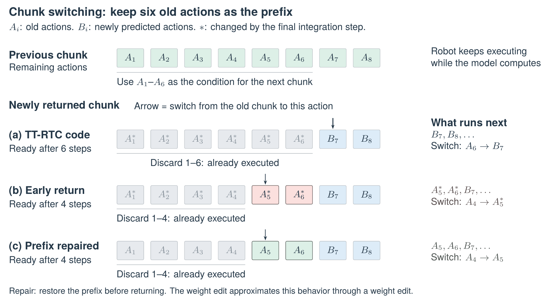
Switching from the old chunk to the new one. The top row shows the old plan’s remaining actions when computation starts; the first six are used as conditions. The three rows below show returned action sequences, with arrows marking where execution resumes after the switch. Gray positions are discarded, and asterisks indicate modifications left by the final sampling integration step. (a) A six-step wait: the old plan reaches \(A_6\) , then switches to \(B_7\) . (b) A four-step wait: the old plan reaches \(A_4\) , but switches to modified \(A_5^*,A_6^*\) (red). (c) After repair, the switch still occurs after \(A_4\) , but continues with unchanged \(A_5,A_6\) (green), followed by new actions \(B_7,B_8\) .
Figure 6. Switching from the old chunk to the new one. The top row shows the old plan’s remaining actions when computation starts; the first six are used as conditions. The three rows below show returned action sequences, with arrows marking where execution resumes after the switch. Gray positions are discarded, and asterisks indicate modifications left by the final sampling integration step. (a) A six-step wait: the old plan reaches A6, then switches to B7. (b) A four-step wait: the old plan reaches A4, but switches to modified A5∗,A6∗ (red). (c) After repair, the switch still occurs after A4, but continues with unchanged A5,A6 (green), followed by new actions B7,B8.

Figure 6(b) shows the problem when the result returns early. Model computation takes only four action steps, and the robot has reached only A4 of the old chunk, so it still needs A5,A6. However, the conditioning prefix still participates in integration updates during flow-matching sampling. With the ten sampling iterations we use, prefix changes made by integrations 1–9 are replaced by the supplied old actions before the next iteration. After the tenth integration, however, the result is returned directly, without another replacement. Consequently, the new result may contain A5∗,A6∗ rather than the planned A5,A6. Switching chunks at this point sends the robot two modified actions, producing a jump. Under the setup in Figure 6(a), the official TT-RTC code discards the entire prefix, so this issue is not exposed.

For deployments requiring IK, we typically reserve a conservatively longer prefix to cover solver-latency fluctuations. Larger fluctuations can also create a larger gap between this reserved length and the latency of a particular inference call. When a result returns early, more conditioning actions remain to be executed. The original OpenWAM [6] implementation uses Mink differential IK wrapped by i2rt, solving quadratic programs (QPs) iteratively. Action decoding, including IK, has a median duration of 22.9 ms and a maximum of 921.2 ms. The subsequently used DLS gate adjusts motion regularization according to the Jacobian’s smallest singular value and limits joint changes; its duration still ranges from a median of 49.3 ms to a maximum of 177.7 ms.

Figure 6(c) shows the repaired transition: even when the new result arrives after A4, the next executed actions are still the planned A5,A6. Opus 5.5’s prefix repair makes the sampling updates for these conditioning actions close to zero, greatly reducing the changes introduced by the final integration step. It edits the time-modulation weights of the action expert’s final normalization layer, final_norm_1.Dense_0.kernel. Under the current setup, its effect is nearly equivalent to executing actions[:6] = condition[:6] before returning: restoring the first six steps to the supplied old actions. Opus approximated this operation by editing parameters.

We subsequently added controls on the same 36 observations (12 local demonstration observations and 24 historical rollout observations), fixing random seeds and sampling steps. We compared shortening the conditioning prefix, using prefix repair alone, and directly restoring the prefix, all without the tempo edit.

Table 9. Prefix-handling controls on 36 identical observations, assuming four steps are discarded in execution. The transition-step distance is the TCP distance from step 4 of the old plan to step 5 of the new plan, taking the larger value across the two arms and then the median across samples. Subsequent-action difference is the RMS relative to the original model over steps 7–38 and 12 joints, averaged across samples.

Method Transition step (mm) Subsequent difference (rad)
Original, 6-step conditioning 19.158 0.000000
Original, 4-step conditioning 4.930 0.002228
Prefix repair only, 6-step conditioning 1.798 0.000375
Code fix: restore 6 steps before return 1.885 0.000000

Table 9 shows that, compared with the original 19.16 mm, the prefix weight edit and the code fix that directly restores the prefix reduce the median transition-step distance to 1.80 and 1.88 mm, respectively, with very small changes to subsequent actions. This supports their approximate equivalence for prefix repair. Shortening the conditioning prefix to four steps also improves this particular comparison, but does not eliminate the same issue when actual latency is shorter than the conditioning length.

By editing time-modulation weights to make updates to the conditioning prefix close to zero, Opus repaired in parameter space a bug left unhandled by the official public code: when actual latency is shorter than the preset prefix, conditioning actions altered by sampling updates may still enter the execution sequence. This prefix protection is especially important for deployments requiring IK, where a margin must be reserved for latency fluctuations. We did not specify this defect; Opus discovered it during its research and produced a parameter-level repair under the constraint of leaving inference code unchanged.

3.3 Mechanism Analysis: Which Attention Changes Preserve the Progress Gain?#

We compared the original model, the direct RoPE teacher, and the tempo-edited model on the same eight bottle-task observations, fixing the initial noise, RTC conditions, and number of sampling steps, with prefix repair disabled. First, the tempo-edited model’s attention to context was closer to the teacher’s: its distributional distance, measured by JSD, was 0.00173, below its distance of 0.00792 from the original model (lower means more similar). This supports that fitting preserved part of the position intervention’s internal effect.
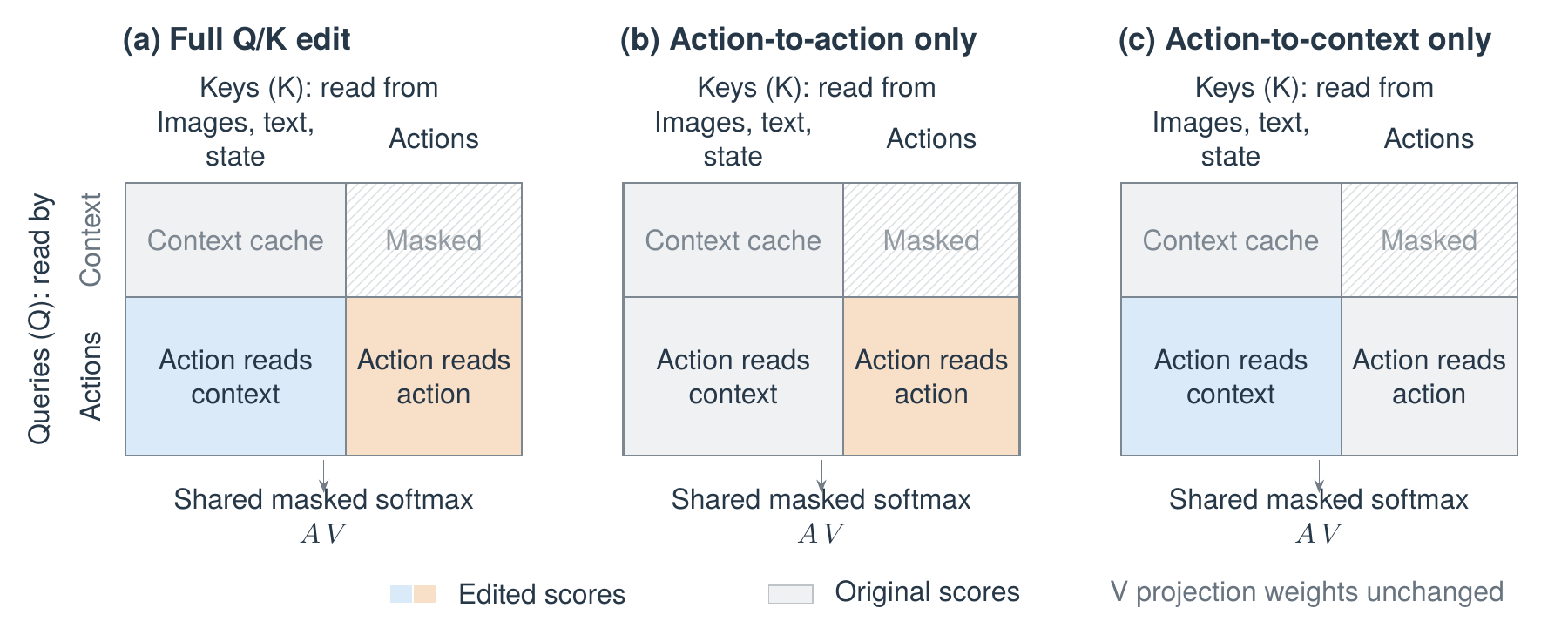
Attention-score interventions before the shared masked softmax. Rows are queries; columns are keys. Blue: actions reading context. Orange: actions reading actions. Gray: original scores. The upper-right block is masked. Colors denote interventions, not measured magnitudes.
Figure 7. Attention-score interventions before the shared masked softmax. Rows are queries; columns are keys. Blue: actions reading context. Orange: actions reading actions. Gray: original scores. The upper-right block is masked. Colors denote interventions, not measured magnitudes.

Figure 7 marks two regions: the lower-right block contains actions reading actions, and the lower-left block contains actions reading images, text, and state. At each layer, using the same current hidden features X, we compute projections with the original (r=0) and edited (r=E) Q/K weights according to Equation (7) and apply the original RoPE, obtaining the pre-softmax scores: Lijr=(Qir)TKjrd,Lr=[Lctxr∣Lactr],r∈{0,E}.(18) Here, i is an action query, j is a key, and d=256; ctx denotes images, text, and state, while act denotes actions. Cached context keys remain unchanged. The two regional interventions are Aact-only=softmax([Lctx0∣LactE]+M),Actx-only=softmax([LctxE∣Lact0]+M).(19) M is the original attention mask (0 at readable positions and −∞ at masked positions). The combined scores are normalized together, followed by AV and the remaining forward pass; V projection weights remain unchanged. Because the softmax denominator is shared, changing one block’s scores can also change the other block’s probabilities.

Table 10. Effects of attention-route interventions on predicted actions, reported as medians over eight inputs. Progress is measured along the original path at steps 21 and 37. All variants use the same arms, selected by at least 15 mm of cumulative motion in the original predictions. Prefix repair is disabled throughout, and jerk is measured within chunks. These are geometric quantities of offline plans, not measured completion times.

Intervention Progress at 21 Progress at 37 Deviation (mm) Jerk ratio
Original 1.000 1.000 — 1.000
Direct RoPE teacher 1.203 1.101 1.012 1.105
Full tempo edit 1.227 1.140 1.028 1.289
Action-key scores only 1.178 1.087 1.100 1.249
Image and prompt/state scores only 1.057 1.039 0.484 0.981

Table 10 shows that the step-37 progress ratio changes from 1.140 with the full tempo edit to 1.087 with the action-only intervention and 1.039 with the context-only intervention. Intervening on scores between actions preserves more of the offline progress gain.

Closing Thoughts#

We expected a moment of magic: Claude would intuitively change a few weights, and the robot would move faster. That is not what happened. We believe the key to this Weight Editing result was the Frontier Model’s AutoResearch ability: understanding mechanisms, finding problems, testing hypotheses, and revising its approach after failure. Its understanding of parameter space made the edits possible; the research process helped it find edits worth making.

This raises a more important question: as Frontier Models increasingly internalize robotics knowledge, how will the next generation, and the generations beyond it, change the way we ask questions, test ideas, and advance research? This case cannot yet provide an answer, but it makes these questions concrete and leaves us excited about what comes next. As models take on more exploration and validation, we need to think more carefully: how can we distill robotics needs into research tasks suited to AutoResearch? And how can we identify more meaningful scientific or engineering problems?

We hope this article offers a glimpse into research on Frontier Models for Robotics.

References

  1. Rikiya Takehi, Jayden Teoh, Alex Zhang, Omar Khattab. Sparks of Weight-Space Programming: LLMs can natively read & write neural network weights. MIT CSAIL, 2026. https://rikiyat.github.io/blog/weight-space-programming/.

  2. Physical Intelligence et al. π0.5: a Vision-Language-Action Model with Open-World Generalization. arXiv:2504.16054, 2025. https://arxiv.org/abs/2504.16054.

  3. Jianlin Su et al. RoFormer: Enhanced Transformer with Rotary Position Embedding. arXiv:2104.09864. https://arxiv.org/abs/2104.09864.

  4. Kevin Black, Allen Z. Ren, Michael Equi, Sergey Levine. Training-Time Action Conditioning for Efficient Real-Time Chunking. arXiv:2512.05964v2. https://arxiv.org/html/2512.05964v2.

  5. Physical Intelligence. real-time-chunking-kinetix, commit 9296f31d62d5. https://github.com/Physical-Intelligence/real-time-chunking-kinetix. We inspected src/model.py and src/eval_flow.py.

  6. Yuran Wang et al. OpenWAM: An Open, Modular Exploration Towards Systematic World-Action Model Pretraining. arXiv:2609.07398, 2026. https://arxiv.org/abs/2609.07398.

BibTeX

@misc{gong2026roboticsweightediting,
  author = {Gong, Ziyang and Zheng, Kaifeng and Huang, Yingrui and
            Chen, Wendi and Tian, Jiaguo and Yang, Junkai and
            Liu, Minghuan and Yang, Zhenjie},
  title = {{We Asked Opus-5.5 to Edit $\pi_{0.5}$'s Weights.
            AutoResearch Made It Happen.}},
  year = {2026},
  url = {https://cuzyoung.github.io/robotics-weight-editing/en/}
}

Original research prompt
Download English TXT ↓

# Research Task: Autonomous Weight-Space Acceleration for π₀.₅

## Background

We currently have two trained VLA policies:

1. π₀.₅ Latest
2. π₀.₅ Training-Time RTC

Both policies can already perform some manipulation tasks on a real robot, but there is still room to improve their execution speed.

I would like to explore the **Weight-Space Programming** approach recently proposed by MIT: having a frontier model directly understand and modify neural network weights to improve a VLA policy's real-world execution speed without conventional gradient-based training.

Reference:

https://rikiyat.github.io/blog/weight-space-programming/

This is an exploratory Weight-Space Programming research project, rather than a conventional inference acceleration, runtime optimization, or fine-tuning task.

**The core goal is to make the robot's actions noticeably faster while preserving the original policy's motion smoothness, stability, and task success rate.**

The motion does not need to be smoother than the original, but the speed improvement must not introduce noticeable stuttering, shaking, abrupt stops, or discontinuities.

## Objective

**Can we directly accelerate a pretrained VLA policy through weight-space editing, without gradient-based training, while preserving its original motion smoothness and task performance?**

The aim is to make the policy generate more efficient action trajectories by directly analyzing and modifying π₀.₅'s weights.

Specific goals:

1. **Faster Execution**: Significantly reduce the time the real robot needs to complete a task.
2. **Preserved Smoothness**: Keep motion smoothness at least close to that of the original policy, without noticeably increasing stuttering, shaking, or action discontinuities.
3. **Preserved Success Rate**: Preserve or improve the original task success rate as much as possible.
4. **Minimal Weight Modification**: Modify as few parameters as possible.
5. **No Runtime Overhead**: Introduce no additional inference modules or deployment latency.
6. **Generalization**: Investigate whether the acceleration generalizes across tasks, initial states, and object positions.

Prioritize improvements in actual robot execution speed over simply changing action magnitudes.

## Phase 1: Autonomous Investigation

Begin by independently exploring the current codebase, model architecture, and experiment records.

Locate:

- The model weights and configuration for π₀.₅ Latest.
- The model weights and configuration for π₀.₅ Training-Time RTC.
- Recent real-robot execution logs.
- The corresponding robot states, action trajectories, execution times, task success rates, and videos.
- The current policy's inference pipeline, action expert architecture, and flow matching implementation.
- The current runtime's action chunking, RTC, action interpolation, smoothing, and execution mechanisms.

Prioritize Training-Time RTC.

Focus on the following questions:

- Which stages account for most of the current policy's task execution time?
- Are there unnecessary pauses, waits, or periods of slow motion?
- Are there action paths that could be shortened?
- Are there velocity discontinuities between action chunks?
- Is execution speed primarily limited by the policy's predictions or by the runtime/controller?
- Is the current policy already close to the hardware's safe motion speed limits?
- Can execution efficiency be improved by changing the distribution of actions produced by the policy?

Pay particular attention to the following:

**Do not equate inference latency reduction with robot execution acceleration.**

Clearly distinguish between:

1. Model Inference Latency
2. Action Chunk Generation
3. Runtime Scheduling / Execution
4. Robot Motion Duration
5. End-to-end Task Completion Time

Our primary goal is to improve items 4 and 5.

If the main bottleneck lies in the runtime, report that honestly. However, this study should still prioritize exploring the potential of weight-space editing.

## Phase 2: Safe Model Duplication

Before running any experiments:

1. Locate the original Training-Time RTC checkpoint.
2. Create a separate experimental copy.
3. Record the original checkpoint's hash, configuration, and version.
4. Apply all weight edits only to the experimental copy.
5. Establish mechanisms for saving, loading, comparing, and rolling back weight patches.
6. Write all new experiment outputs to separate directories.

**Never overwrite, delete, or modify any original model weights, configurations, experiment records, or data.**

Do not modify π₀.₅ Latest for now.

Consider transferring the approach to Latest only after making clear progress on Training-Time RTC.

If loading the model could write to the original checkpoint, eliminate that risk first.

## Phase 3: Weight-Space Investigation

Follow the research approach described in MIT's Weight-Space Programming work:

**Inspect → Hypothesize → Edit → Evaluate → Iterate**

You may independently design analysis tools, including:

- Weight Inspection
- Activation Inspection
- Action Expert Investigation
- Flow Matching Trajectory Analysis
- Layer-wise Sensitivity Analysis
- Sparse Weight Editing
- Low-rank Weight Editing
- Forward-only Parameter Search
- Action Distribution Analysis
- Motion Smoothness Analysis

Focus on the following questions:

### 3.1 Can we identify speed-related directions in weight space?

Can we identify parameter directions in the action expert or other relevant modules that affect the robot's motion speed?

For example:

- Do certain parameters affect action magnitudes?
- Do certain parameters affect slow phases of a trajectory?
- Do certain parameters affect the temporal distribution of action chunks?
- Do certain parameters affect acceleration and deceleration behavior?

Try to identify weight-space directions that change execution speed while preserving the action targets and overall trajectory shape as much as possible.

### 3.2 Can we accelerate motion without introducing jerk?

Can localized weight edits make the policy generate faster trajectories that remain continuous?

We would like to achieve:

\[
T_{\mathrm{edited}} < T_{\mathrm{original}}
\]

while satisfying:

\[
J_{\mathrm{edited}}
\approx
J_{\mathrm{original}}
\]

where:

- \(T\) denotes actual task completion time.
- \(J\) denotes trajectory jerk or another measure of motion smoothness.

Note that the absolute value of jerk depends on motion speed and timescale, so raw jerk values alone cannot determine whether motion is smoother.

Evaluate velocity, acceleration, jerk, action discontinuities, and actual execution behavior together.

### 3.3 Can we preserve task semantics while accelerating execution?

The policy should still complete the original manipulation tasks correctly.

For example:

- Grasp locations must not shift noticeably as a result of acceleration.
- The robot must still decelerate appropriately when approaching a target.
- Contact with objects must not cause pronounced impacts.
- The timing of gripper opening and closing must remain appropriate.
- Task completion detection must not trigger prematurely.

**We are aiming for more efficient motion, rather than simply multiplying every action by a factor greater than 1.**

## Phase 4: Autonomous Weight Editing

Independently perform weight-space editing on the separate experimental copy of Training-Time RTC.

You may explore different approaches, including:

- Sparse Parameter Modification
- Low-rank Weight Updates
- Selected Layer Editing
- Action Expert Weight Surgery
- Behavior-related Circuit Editing
- Forward-only Weight-Space Search

You do not need to commit to a particular method in advance.

You may propose new editing strategies based on the model architecture, weight distributions, and experimental results.

However, you must follow this restriction:

**Do not use backpropagation, gradient descent, optimizer steps, LoRA fine-tuning, or any other gradient-based training methods.**

You may:

- Read model parameters.
- Analyze activations.
- Run forward passes.
- Compare the action outputs of different weight patches.
- Use gradient-free search methods.
- Iterate independently based on experimental feedback.

For every edit, record:

1. The layers/modules modified.
2. The number and percentage of parameters modified.
3. The exact form of the weight patch.
4. Action predictions before and after the edit.
5. Velocity, acceleration, and jerk before and after the edit.
6. Estimated task completion time before and after the edit.
7. Potential effects on task success rate and motion stability.

Do not assume that any particular weight-editing method will work.

Failure is acceptable; use failed experiments to adjust the research direction.

## Phase 5: Evaluation

Prioritize validation using existing experimental records and offline data.

If a simulation environment is available, you may also perform closed-loop evaluation.

Do not automatically start real-robot execution without my explicit confirmation.

### 5.1 Baselines

Compare at least the following:

1. Original Training-Time RTC
2. Original Policy + Action Scaling
3. Original Policy + Trajectory Time Scaling
4. Random Weight Editing
5. Proposed Weight-Space Editing

Action Scaling and Trajectory Time Scaling are only control experiments and must not be presented as Weight-Space Programming.

You may also independently add other reasonable baselines for speed optimization.

### 5.2 Metrics

**Execution Efficiency**

- End-to-end Task Completion Time
- Robot Motion Duration
- Average EEF Velocity
- Peak EEF Velocity
- Idle / Pause Duration
- Trajectory Length

**Motion Smoothness**

- Velocity Continuity
- Acceleration Continuity
- Jerk
- Action Chunk Boundary Discontinuity
- Oscillation Frequency
- Unexpected Stops

**Task Performance**

- Task Success Rate
- Final Position Error
- Grasp / Placement Accuracy
- Collision Rate
- Contact Stability

**Weight Editing**

- Number of Modified Parameters
- Percentage of Modified Parameters
- Weight Patch Norm
- Inference Latency
- Regression on Other Tasks

### 5.3 Success Criteria

Prioritize exploring whether the following can be achieved:

- Reduce task completion time by **20%–30%**.
- Keep the task success rate at least as high as the original, allowing for statistical uncertainty.
- Maintain motion smoothness close to the original.
- Introduce no noticeable new stuttering, oscillations, or unexpected stops.
- Do not increase model inference latency.
- Require no additional runtime controller.

20%–30% is an exploratory target and must not be treated as a mandatory requirement.

Even if the result is only a stable 5%–10% speedup, retain it as long as the improvement can be shown to come from weight editing and there is no noticeable performance degradation.

Without sufficient closed-loop evaluation, do not directly interpret improvements in offline action predictions as improvements in real execution speed.

## Phase 6: Weight-Space Speed Control

If the preceding experiments make progress, you can further explore a question with greater research value:

**Can we discover a controllable speed direction in the weight space of a pretrained VLA?**

Suppose there is a parameter direction:

\[
\Delta\theta_{\mathrm{speed}}
\]

Can we then use:

\[
\theta'=\theta+\alpha\Delta\theta_{\mathrm{speed}}
\]

to control the policy's motion speed?

For example:

| α | Expected Behavior |
|---|---|
| 0 | Original Policy |
| 0.25 | Slightly Faster |
| 0.5 | Moderately Faster |
| 1.0 | Significantly Faster |

Validate the following:

1. Does speed vary approximately monotonically with α?
2. Do different values of α preserve similar motion trajectories?
3. Is there a noticeable trade-off between speed and smoothness?
4. Can this direction generalize to different tasks?
5. Is there a safe and stable range of α?

Finding a controllable, reusable speed direction would have greater research value than simply obtaining a faster checkpoint.

## Research Principles

This is an open-ended autonomous research task.

You may independently:

- Read the code and model architecture.
- Analyze weights and activations.
- Write experimental scripts.
- Run model inference.
- Construct and test weight patches.
- Design new diagnostic experiments.
- Revise research hypotheses.
- Try different weight-space editing methods.

You do not need to ask me for confirmation at every step.

However, you must ensure the following:

1. Keep the original checkpoint and experimental data completely safe.
2. Do not use gradient-based training.
3. Do not disguise runtime optimization as weight editing.
4. Do not disguise simple action scaling as a new research method.
5. Do not sacrifice task success rate or motion stability to improve speed.
6. Do not start a real robot without authorization.
7. All conclusions must be supported by reproducible experimental evidence.

Pay particular attention to the following:

**Greater action magnitudes do not mean faster task completion.**

If the robot's actuators have speed limits, control delays, or action saturation, simply scaling up actions may lead to more severe oscillations and task failures.

You must assess whether the speed improvement holds by examining the actual execution pipeline.

## Expected Deliverables

The desired final deliverables are:

1. A separate Training-Time RTC checkpoint with edited weights.
2. The corresponding weight patch file and reproducible code.
3. A comparison of action trajectories from the original and modified policies.
4. Evaluation results for execution speed, motion smoothness, and task performance.
5. Research conclusions on whether weight-space acceleration is effective.
6. If it is effective, an analysis of which parameter modifications caused the speed changes.
7. If it is ineffective, an analysis of the technical bottlenecks and directions worth exploring next.
8. If a controllable speed direction is discovered, the corresponding parameter patch and control experiments.

Do not make parameter modifications unsupported by evidence merely to deliver a modified checkpoint. If no effective result can be obtained, report that honestly.

## Final Instruction

**Start with Training-Time RTC.**

Autonomously investigate the model architecture, weights, action generation process, and existing execution logs.

Explore whether direct weight-space editing can produce faster robotic motion while preserving the original policy's smoothness and task performance.

Preserve all original artifacts.

Do not overwrite any existing checkpoint.

Do not use gradient-based training.

Do not modify the production runtime or robot controller.

Iterate based on evidence, and prioritize measurable improvements over speculative claims.

**The ultimate goal is not merely to make the robot move faster, but to discover whether execution speed can be directly programmed into the weight space of a pretrained VLA.**
